Formatting data
Remarkable Charts will use any formatting applied to the data in Excel.
Here are some common examples.
Show or hide the thousands separator
Select the cells that you want to format.
On the Home tab, click the Dialog Box Launcher next to Number.
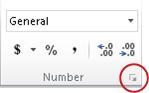
On the Number tab, in the Category list, click Number.
To display or hide the thousands separator, select or clear the Use 1000 Separator (,) check box.
Tip
To quickly display the thousands separator, you can click Comma Style  in the Number group on the Home tab.
Format a date the way you want
When you enter some text into a cell such as "2/2", Excel assumes that this is a date and formats it according to the default date setting in Control Panel. Excel might format it as "2-Feb". If you change your date setting in Control Panel, the default date format in Excel will change accordingly. If you don’t like the default date format, you can choose another date format in Excel, such as "February 2, 2012" or "2/2/12". You can also create your own custom format in Excel desktop.
Millions and billions
This requires you to create a custom number format.
Compatibility
You can't create custom formats in Excel for the web but if you have the Excel desktop application, you can click the Open in Excel button to open the workbook and create them.
Let's work with this data.
112145
319320
Select the numeric data
On the Home tab, in the Number group, click the Dialog launcher
Select Custom
In the Type list, type a new format in the box.
#,##0,
Your numbers will now show in units of thousands.
112
319
You can indicate a number is measured in thousands by adding to the number syntax.
#,##0,"k"
Your numbers will now show as
112k
319k
Note that you must put double quotes around the letter(s) you use.